Cet article poursuit le travail commencé ici en procédant à une généralisation du modèle utilisé.
Introduction
Cet article est assez technique et est destiné à documenter le calcul de la position d’un salaire dans la distribution des salaires du secteur privé dans notre Observatoire des salaires des enseignants ainsi que sur notre page Où vous trouvez-vous sur l’échelle des salaires ?.
Si vous êtes intéressé par les animations de convergence et la précision obtenue, rendez-vous directement dans la dernière partie de l’article, mais si vous avez quelques bases en analyse numérique et êtes intéressé par le type d’interpolation utilisé, vous pourrez trouver dans ce qui suit quelques indications sur la méthode que nous avons utilisée.
Modèle de fonction de répartition utilisé
Supposons connus  quantiles d’une série statistique.
Notons  ,
,  , …
, …  les points correspondants par lesquels doit passer la courbe de la fonction de répartition (les ordonnées sont comprises entre
  et
et  et les abscisses, tout comme les ordonnées, sont classées par ordre croissant).
Plusieurs modèles de fonction de répartition seront ici possibles.
Le choix d’un modèle est conditionné par les valeurs des paramètres suivants :
 : paramètre valant si le polynôme utilisé dans la branche asymptotique gauche est une fonction affine, et valant s’il sagit d’un trinôme du second degré ;
 : paramètre valant si le polynôme utilisé dans la branche asymptotique droite est une fonction affine, et valant s’il sagit d’un trinôme du second degré ;
 : fonction pouvant être l’identité ou bien la fonction
  (logarithme népérien) ; dans le premier cas, les valeurs possibles des quantiles appartiennent à
  , dans le second, elles appartiennent à
  .
.
La fonction de répartition est alors modélisée par la fonction  de classe
  paramétrée par , et (choisis au préalables) ainsi que le vecteur
  contenant
  coefficients (dont les valeurs seront déterminées au cours de l’optimisation), de la forme :
![\[F\left(x;(a,\delta_g,\delta_d,h)\right)=\left\{\begin{array}{ll}\exp\left( a_0 + a_1 h(x) + \delta_g a_2 h(x)^2 \right) & \text{si } x \leq x_0 \\a_{2+\delta_g} + a_{3+\delta_g}h(x) + a_{4+\delta_g}h(x)^2 + a_{5+\delta_g}h(x)^3 & \text{si } x_0 < x \leq x_1 \\\vdots & \vdots \\a_{4i+2+\delta_g} + a_{4i+3+\delta_g}h(x) + a_{4i+4+\delta_g}h(x)^2 + a_{4i+5+\delta_g}h(x)^3 & \text{si } x_{i} < x \leq x_{i+1} \\\vdots & \vdots \\a_{4n-6+\delta_g} + a_{4n-5+\delta_g}h(x) + a_{4n-4+\delta_g}h(x)^2 + a_{4n-3+\delta_g}h(x)^3 & \text{si } x_{n-2} < x \leq x_{n-1} \\1-\exp\left( a_{4n-2+\delta_g} + a_{4n-1+\delta_g}h(x) + \delta_d a_{4n+\delta_g}h(x)^2 \right) & \text{si } x_{n-1} < x \\\end{array}\right. .\]](https://blog.epicycle.fr/wp-content/ql-cache/quicklatex.com-6530be535be5c1ac161efe50b6a75034_l3.png "Rendered by QuickLaTeX.com")
La fonction étant de classe , sa dérivée, la fonction de densité  est de classe
  . Celle-ci s’exprime de la façon suivante :
![\[f\left(x;(a,\delta_g,\delta_d,h)\right)=\left\{\begin{array}{ll}h'(x) \left( a_1 + 2\delta_g a_2 h(x) \right)\exp\left( a_0 + a_1 h(x) + \delta_g a_2 h(x)^2 \right) & \text{si } x \leq x_0 \\h'(x) \left( a_{3+\delta_g} + 2 a_{4+\delta_g}h(x) + 3 a_{5+\delta_g}h(x)^2 \right) & \text{si } x_0 < x \leq x_1 \\\vdots & \vdots \\h'(x) \left( a_{4i+3+\delta_g} + 2 a_{4i+4+\delta_g}h(x) + 3 a_{4i+5+\delta_g}h(x)^2 \right) & \text{si } x_{i} < x \leq x_{i+1} \\\vdots & \vdots \\h'(x) \left( a_{4n-5+\delta_g} + 2 a_{4n-4+\delta_g}h(x) + 3 a_{4n-3+\delta_g}h(x)^2 \right) & \text{si } x_{n-2} < x \leq x_{n-1} \\-h'(x)\left( a_{4n-1+\delta_g} + 2 \delta_d a_{4n+\delta_g}h(x) \right)\exp\left( a_{4n-2+\delta_g} + a_{4n-1+\delta_g}h(x) + \delta_d a_{4n+\delta_g}h(x)^2 \right) & \text{si } x_{n-1} < x \\\end{array}\right. .\]](https://blog.epicycle.fr/wp-content/ql-cache/quicklatex.com-3e8c4a901022a449992f7bbc37be64b1_l3.png "Rendered by QuickLaTeX.com")
Système d’équations à résoudre
Un raccordement  pour en chacun des points permet d’obtenir
  équations (
 pour les raccordements
  à droite et à gauche de chaque point, pour le raccordement
  , et pour le raccordement ).
Afin d’obtenir un système carré, on ajoute une équation de raccordement  sur le point
  lorsque vaut et sur le point
  lorsque vaut , ce qui nous donne un total de équations, égal au nombre de paramètres à déterminer.
Le système à résoudre est alors le suivant :
![\[ \left\{ \begin{array}{l} \begin{array}{lclcl} \text{raccordements } \mathcal{C}^0 \text{ : } & & \\ \exp\left(a_0 + a_1 h(x_0) + \delta_g a_2 h(x_0)^2\right) & - & y_0 & = & 0 \\ a_{2+\delta_g} + a_{3+\delta_g}h(x_0) + a_{4+\delta_g}h(x_0)^2 + a_{5+\delta_g}h(x_0)^3 & - & y_0 & = & 0 \\ & \vdots & & \vdots & \\ a_{4i+2+\delta_g} + a_{4i+3+\delta_g}h(x_i) + a_{4i+4+\delta_g}h(x_i)^2 + a_{4i+5+\delta_g}h(x_i)^3 & - & y_{i} & = & 0 \\ a_{4i+2+\delta_g} + a_{4i+3+\delta_g}h(x_{i+1}) + a_{4i+4+\delta_g}h(x_{i+1})^2 + a_{4i+5+\delta_g}h(x_{i+1})^3 & - & y_{i+1} & = & 0 \\ & \vdots & & \vdots & \\ a_{4n-6+\delta_g} + a_{4n-5+\delta_g}h(x_{n-1}) + a_{4n-4+\delta_g}h(x_{n-1})^2 + a_{4n-3+\delta_g}h(x_{n-1})^3 & - & y_{n-1} & = & 0 \\ 1-\exp\left(a_{4n-2+\delta_g} + a_{4n-1+\delta_g}h(x_{n-1}) + \delta_d a_{4n+\delta_g}h(x_{n-1})^2\right) & - & y_{n-1} & = & 0 \\ \end{array} \\ \\ \begin{array}{lclcl} \text{raccordements } \mathcal{C}^1 \text{ : } & & \\ \left(a_1 + 2\delta_g a_2 h(x_0)\right)\exp\left(a_0 + a_1 h(x_0) + \delta_g a_2 h(x_0)^2\right) & - & \left(a_{3+\delta_g} + 2 a_{4+\delta_g}h(x_0) + 3 a_{5+\delta_g}h(x_0)^2\right) & = & 0 \\ & \vdots & & \vdots & \\ a_{4i-1+\delta_g} + 2 a_{4i+\delta_g}h(x_i) + 3 a_{4i+1+\delta_g}h(x_i)^2 & - & \left(a_{4i+3+\delta_g} + 2 a_{4i+4+\delta_g}h(x_i) + 3 a_{4i+5+\delta_g}h(x_i)^2\right) & = & 0 \\ & \vdots & & \vdots & \\ a_{4n-5+\delta_g} + 2 a_{4n-4+\delta_g}h(x_{n-1}) + 3 a_{4n-3+\delta_g}h(x_{n-1})^2 & + &\left (a_{4n-1+\delta_g} + 2 \delta_d a_{4n+\delta_g}h(x_{n-1})\right)\exp\left(a_{4n-2+\delta_g} + a_{4n-1+\delta_g}h(x_{n-1}) + \delta_d a_{4n+\delta_g}h(x_{n-1})^2\right) & = & 0 \\ \end{array} \\ \\ \begin{array}{lclcl} \text{raccordements } \mathcal{C}^2 \text{ : } & & \\ \left(a_1^2 + 2\delta_g a_2 \left( 1 + 2 a_1 h(x_0) + 2 a_2 h(x_0)^2 \right) \right)\exp\left(a_0 + a_1 h(x_0) + \delta_g a_2 h(x_0)^2\right) & - & \left( 2 a_{4+\delta_g} + 6 a_{5+\delta_g}h(x_0) \right) & = & 0 \\ & \vdots & & \vdots & \\ 2 a_{4i+\delta_g} + 6 a_{4i+1+\delta_g}h(x_i) & - & \left( 2 a_{4i+4+\delta_g} + 6 a_{4i+5+\delta_g}h(x_i) \right) & = & 0 \\ & \vdots & & \vdots & \\ 2 a_{4n-4+\delta_g} + 6 a_{4n-3+\delta_g}h(x_{n-1}) & + &\left ( a_{4n-1+\delta_g}^2 + 2 \delta_d a_{4n+\delta_g} \left( 1 + 2 a_{4n-1+\delta_g}h(x_{n-1}) + 2 a_{4n+\delta_g}h(x_{n-1})^2 \right) \right)\exp\left(a_{4n-2+\delta_g} + a_{4n-1+\delta_g}h(x_{n-1}) + \delta_d a_{4n+\delta_g}h(x_{n-1})^2\right) & = & 0 \\ \end{array} \\ \\ \begin{array}{lcl} \text{raccordements } \mathcal{C}^3 \text{ (ajoutés au système seulement si $\delta_g=1$ pour le premier et si $\delta_d=1$ pour le second) : } & & \\ \left(a_1^3 + 2\delta_g a_2 \left( 3 a_1 + (3 a_1^2 + 6 a_2) h(x_0) + 6 a_1 a_2 h(x_0)^2 + 4 a_2^2 h(x_0)^3 \right) \right)\exp\left(a_0 + a_1 h(x_0) + \delta_g a_2 h(x_0)^2\right) - 6 a_{5+\delta_g} & = & 0 \\ 6 a_{4n-3+\delta_g} + \left ( a_{4n-1+\delta_g}^3 + 2 \delta_d a_{4n+\delta_g} \left( 3 a_{4n-1+\delta_g} + (3 a_{4n-1+\delta_g}^2 + 6 a_{4n+\delta_g})h(x_{n-1}) + 6 a_{4n-1+\delta_g}a_{4n+\delta_g}h(x_{n-1})^2 + 4 a_{4n+\delta_g}^2 h(x_{n-1})^3\right) \right)\exp\left(a_{4n-2+\delta_g} + a_{4n-1+\delta_g}h(x_{n-1}) + \delta_d a_{4n+\delta_g}h(x_{n-1})^2\right) & = & 0 \\ \end{array} \end{array} \right. . \]](https://blog.epicycle.fr/wp-content/ql-cache/quicklatex.com-8d43dd236c661d072998d619062a36c5_l3.png "Rendered by QuickLaTeX.com")
Ce système étant non linéaire, nous procéderons à sa résolution approchée à l’aide de la méthode de Newton. Pour cela, la matrice jacobienne correspondante sera nécessaire.
De plus, la fonction objectif dont on cherche un zéro est donnée par les membres de gauche des égalités du système d’équations.
Matrice jacobienne
Dans ce qui suit, on note :  .
.
Voici les  premières colonnes de la matrice jacobienne, elles contiennent les dérivées partielles par rapport aux paramètres
  à
à  :
:
![\[ \left( \begin{array}{*2{>{\displaystyle}c}|*1{>{\displaystyle}c}|*4{>{\displaystyle}c}|*1{>{\displaystyle}c}} E_1 & E_2 & E_3 & 0 & 0 & 0 & 0 & \multirow{4}{*}{\text{$(\ast)$}} \\ \multicolumn{3}{c|}{\multirow{3}{*}{\text{$(0)$}}} & 1 & x_0 & x_0^2 & x_0^3 \\ \multicolumn{3}{c|}{} & 1 & x_1 & x_1^2 & x_1^3 \\ \multicolumn{3}{c|}{} & \multicolumn{4}{c|}{\text{$(0)$}} \\ \hline E_4 & E_5 & E_6 & 0 & -1 & -2x_0 & -3x_0^2 & \multirow{3}{*}{\text{$(\ast)$}} \\ \multicolumn{3}{c|}{\multirow{2}{*}{\text{$(0)$}}} & 0 & 1 & 2x_1 & 3x_1^2 \\ \multicolumn{3}{c|}{} & \multicolumn{4}{c|}{\text{$(0)$}} \\ \hline E_7 & E_8 & E_9 & 0 & 0 & -2 & -6x_0 & \multirow{3}{*}{\text{$(\ast)$}} \\ \multicolumn{3}{c|}{\multirow{2}{*}{\text{$(0)$}}} & 0 & 0 & 2 & 6x_1 \\ \multicolumn{3}{c|}{} & \multicolumn{4}{c|}{\text{$(0)$}} \\ \hline E_{10} & E_{11} & E_{12} & 0 & 0 & 0 & -6 & \multirow{2}{*}{\text{$(\ast)$}} \\ $0$ & $0$ & $0$ &$0$ & $0$ & $0$ & $0$ \end{array} \right). \]](https://blog.epicycle.fr/wp-content/ql-cache/quicklatex.com-faa2632bc97e5fcb1b6ba9d77654f3cc_l3.png "Rendered by QuickLaTeX.com")
Avec :
![\[ \begin{split} E_1 =& \exp(P_0(h(x_0))) , \\ E_2 =& h(x_0) \exp(P_0(h(x_0))) , \\ E_3 =& \delta_g h(x_0)^2 \exp(P_0(h(x_0))) , \\ E_4 =& \left( a_1 + 2 \delta_g a_2 h(x_0) \right) \exp\left(P_0(h(x_0))\right) , \\ E_5 =& \left( 1 + a_1 h(x_0) + 2 \delta_g a_2 h(x_0)^2 \right) \exp\left(P_0(h(x_0))\right) , \\ E_6 =& \delta_g h(x_0) \left( 2 + a_1 h(x_0) + 2 a_2 h(x_0)^2 \right) \exp\left(P_0(h(x_0))\right) , \\ E_7 =& \left( a_1^2 + 2 \delta_g a_2 \left( 1 + 2 a_1 h(x_0) + 2 a_2 h(x_0)^2 \right) \right) \exp\left(P_0(h(x_0))\right) , \\ E_8 =& \left( 2 a_1 + \left( a_1^2 + 6 \delta_g a_2 \right) h(x_0) + 4 \delta_g a_1 a_2 h(x_0)^2 + 4 \delta_g a_2^2 h(x_0)^3 \right) \exp\left(P_0(h(x_0))\right) , \\ E_9 =& \delta_g \left( 2 + 4 a_1 h(x_0) + \left( 10 a_2 + a_1^2 \right) h(x_0)^2 + 4 a_1 a_2 h(x_0)^3 + 4 a_2^2 h(x_0)^4 \right) \exp\left(P_0(h(x_0))\right) , \\ E_{10} =& \left( a_1^3 + 2 \delta_g a_2 \left( 3 a_1 + \left( 3 a_1^2 + 6 a_2 \right) h(x_0) + 6 a_1 a_2 h(x_0)^2 + 4 a_2^2 h(x_0)^3 \right) \right) \exp\left(P_0(h(x_0))\right) , \\ E_{11} =& \left( 3 a_1^2 + 6 \delta_g a_2 + (a_1^3 + 18 \delta_g a_1 a_2 ) h(x_0) + 6 \delta_g a_2 \left( a_1^2 + 4 a_2 \right) h(x_0)^2 + 12 \delta_g a_1 a_2^2 h(x_0)^3 + 8 \delta_g a_2^3 h(x_0)^4 \right) \exp\left(P_0(h(x_0))\right) , \\ E_{12} =& \delta_g \left( 6 a_1 + 6 (a_1^2 + 4 a_2 ) h(x_0) + a_1 \left( a_1^2 + 30 a_2 \right) h(x_0)^2 + 6 a_2 \left( a_1^2 + 6 a_2 \right) h(x_0)^3 + 12 a_1 a_2^2 h(x_0)^4 + 8 a_2^3 h(x_0)^5 \right) \exp\left(P_0(h(x_0))\right). \end{split} \]](https://blog.epicycle.fr/wp-content/ql-cache/quicklatex.com-d716d7ec23e246cc3fbf42cf03fd6a7c_l3.png "Rendered by QuickLaTeX.com")
Pour tout  , voici les colonnes
  à
à  de la matrice jacobienne, elles contiennent les dérivées partielles par rapport aux paramètres
  à
à  :
:
![\[ \left( \begin{array}{*1{>{\displaystyle}c}|*4{>{\displaystyle}c}|*4{>{\displaystyle}c}|*4{>{\displaystyle}c}|*1{>{\displaystyle}c}} \multirow{9}{*}{\text{$(\ast)$}} & \multicolumn{4}{c|}{\text{$(0)$}} & \multicolumn{4}{c|}{\multirow{3}{*}{\text{$(0)$}}} & \multicolumn{4}{c|}{\multirow{5}{*}{\text{$(0)$}}} & \multirow{9}{*}{\text{$(\ast)$}} \\ & 1 & h(x_{k-2}) & h(x_{k-2})^2 & h(x_{k-2})^3 & \multicolumn{4}{c|}{} & \multicolumn{4}{c|}{} & \\ & 1 & h(x_{k-1}) & h(x_{k-1}^2) & h(x_{k-1}^3) & \multicolumn{4}{c|}{} & \multicolumn{4}{c|}{} & \\ & \multicolumn{4}{c|}{\multirow{5}{*}{\text{$(0)$}}} & 1 & h(x_{k-1}) & h(x_{k-1})^2 & h(x_{k-1})^3 & \multicolumn{4}{c|}{} & \\ & \multicolumn{4}{c|}{} & 1 & h(x_{k}) & h(x_{k})^2 & h(x_{k})^3 & \multicolumn{4}{c|}{} & \\ & \multicolumn{4}{c|}{} & \multicolumn{4}{c|}{\multirow{2}{*}{\text{$(0)$}}} & 1 & h(x_{k}) & h(x_{k})^2 & h(x_{k})^3 & \\ & \multicolumn{4}{c|}{} & \multicolumn{4}{c|}{} & 1 & h(x_{k+1}) & h(x_{k+1})^2 & h(x_{k+1})^3 & \\ & \multicolumn{4}{c|}{} & \multicolumn{4}{c|}{} & \multicolumn{4}{c|}{\text{$(0)$}} & \\ \hline \multirow{6}{*}{\text{$(\ast)$}} & \multicolumn{4}{c|}{\text{$(0)$}} & \multicolumn{4}{c|}{\multirow{2}{*}{\text{$(0)$}}} & \multicolumn{4}{c|}{\multirow{3}{*}{\text{$(0)$}}} & \multirow{6}{*}{\text{$(\ast)$}} \\ & 0 & -1 & -2h(x_{k-2}) & -3h(x_{k-2})^2 & \multicolumn{4}{c|}{} & \multicolumn{4}{c|}{} & \\ & 0 & 1 & 2h(x_{k-1}) & 3h(x_{k-1})^2 & 0 & -1 & -2h(x_{k-1}) & -3h(x_{k-1})^2 & \multicolumn{4}{c|}{} & \\ & \multicolumn{4}{c|}{\multirow{3}{*}{\text{$(0)$}}} & 0 & 1 & 2h(x_{k}) & 3h(x_{k})^2 & 0 & -1 & -2h(x_{k}) & -3h(x_{k})^2 & \\ & \multicolumn{4}{c|}{} & \multicolumn{4}{c|}{\multirow{2}{*}{\text{$(0)$}}} & 0 & 1 & 2h(x_{k+1}) & 3h(x_{k+1})^2 & \\ & \multicolumn{4}{c|}{} & \multicolumn{4}{c|}{} & \multicolumn{4}{c|}{\text{$(0)$}} & \\ \hline \multirow{6}{*}{\text{$(\ast)$}} & \multicolumn{4}{c|}{\text{$(0)$}} & \multicolumn{4}{c|}{\multirow{2}{*}{\text{$(0)$}}} & \multicolumn{4}{c|}{\multirow{3}{*}{\text{$(0)$}}} & \multirow{6}{*}{\text{$(\ast)$}} \\ & 0 & 0 & -2 & -6h(x_{k-2}) & \multicolumn{4}{c|}{} & \multicolumn{4}{c|}{} & \\ & 0 & 0 & 2 & 6h(x_{k-1}) & 0 & 0 & -2 & -6h(x_{k-1}) & \multicolumn{4}{c|}{} & \\ & \multicolumn{4}{c|}{\multirow{3}{*}{\text{$(0)$}}} & 0 & 0 & 2 & 6h(x_{k}) & 0 & 0 & -2 & -6h(x_{k}) & \\ & \multicolumn{4}{c|}{} & \multicolumn{4}{c|}{\multirow{2}{*}{\text{$(0)$}}} & 0 & 0 & 2 & 6h(x_{k+1}) & \\ & \multicolumn{4}{c|}{} & \multicolumn{4}{c|}{} & \multicolumn{4}{c|}{\text{$(0)$}} & \\ \hline \multirow{2}{*}{\text{$(\ast)$}} & 0 & 0 & 0 & 0 & 0 & 0 & 0 & 0 & 0 & 0 & 0 & 0 & \multirow{2}{*}{\text{$(\ast)$}} \\ & 0 & 0 & 0 & 0 & 0 & 0 & 0 & 0 & 0 & 0 & 0 & 0 & \\ \end{array} \right). \]](https://blog.epicycle.fr/wp-content/ql-cache/quicklatex.com-b473b7b5093e8421ab3d3addf95c9918_l3.png "Rendered by QuickLaTeX.com")
Dans ce qui suit, on note  .
.
Voici les  dernières colonnes de la matrice jacobienne, elles contiennent les dérivées partielles par rapport aux paramètres
  à
à  :
:
![\[ \left( \begin{array}{*1{>{\displaystyle}c}|*4{>{\displaystyle}c}|*2{>{\displaystyle}c}|*1{>{\displaystyle}c}} \multirow{4}{*}{\text{$(\ast)$}} & \multicolumn{4}{c|}{\text{$(0)$}} & \multicolumn{2}{c}{\multirow{3}{*}{\text{$(0)$}}} \\ & 1 & x_{n-2} & x_{n-2}^2 & x_{n-2}^3 & \multicolumn{2}{c}{} \\ & 1 & x_{n-1} & x_{n-1}^2 & x_{n-1}^3 & \multicolumn{2}{c}{} \\ & 0 & 0 & 0 & 0 & E'_{1} & E'_{2} & E'_{3} \\ \hline \multirow{3}{*}{\text{$(\ast)$}} & \multicolumn{4}{c|}{\text{$(0)$}} & \multicolumn{2}{c}{\multirow{2}{*}{\text{$(0)$}}} \\ & 0 & -1 & -2x_{n-2} & -3x_{n-2}^2 & \multicolumn{2}{c}{} \\ & 0 & 1 & 2x_{n-1} & 3x_{n-1}^2 & E'_{4} & E'_{5} & E'_{6} \\ \hline \multirow{3}{*}{\text{$(\ast)$}} & \multicolumn{4}{c|}{\text{$(0)$}} & \multicolumn{2}{c}{\multirow{2}{*}{\text{$(0)$}}} \\ & 0 & 0 & -2 & -6x_{n-2} & \multicolumn{2}{c}{} \\ & 0 & 0 & 2 & 6x_{n-1} & E'_{7} & E'_{8} & E'_{9} \\ \hline \multirow{2}{*}{\text{$(\ast)$}} & 0 & 0 & 0 & 0 & 0 & 0 & 0 \\ & 0 & 0 & 0 & 6 & E'_{10} & E'_{11} & E'_{12} \\ \end{array} \right). \]](https://blog.epicycle.fr/wp-content/ql-cache/quicklatex.com-e1cbddb73424fb13cd410efa985971b9_l3.png "Rendered by QuickLaTeX.com")
Avec :
![\[ \begin{split} E'_1 =& -\exp(P_{4n-2+\delta_g}(h(x_{n-1}))) , \\ E'_2 =& -h(x_{n-1}) \exp(P_{4n-2+\delta_g}(h(x_{n-1}))) , \\ E'_3 =& -\delta_d h(x_{n-1})^2 \exp(P_{4n-2+\delta_g}(h(x_{n-1}))) , \\ E'_4 =& \left( a_{4n-1+\delta_g} + 2 \delta_d a_{4n+\delta_g} h(x_{n-1}) \right) \exp\left(P_{4n-2+\delta_g}(h(x_{n-1}))\right) , \\ E'_5 =& \left( 1 + a_{4n-1+\delta_g} h(x_{n-1}) + 2 \delta_d a_{4n+\delta_g} h(x_{n-1})^2 \right) \exp\left(P_{4n-2+\delta_g}(h(x_{n-1}))\right) , \\ E'_6 =& \delta_d h(x_{n-1}) \left( 2 + a_{4n-1+\delta_g} h(x_{n-1}) + 2 a_{4n+\delta_g} h(x_{n-1})^2 \right) \exp\left(P_{4n-2+\delta_g}(h(x_{n-1}))\right) , \\ E'_7 =& \left( a_{4n-1+\delta_g}^2 + 2 \delta_d a_{4n+\delta_g} \left( 1 + 2 a_{4n-1+\delta_g} h(x_{n-1}) + 2 a_{4n+\delta_g} h(x_{n-1})^2 \right) \right) \exp\left(P_{4n-2+\delta_g}(h(x_{n-1}))\right) , \\ E'_8 =& \left( 2 a_{4n-1+\delta_g} + \left( a_{4n-1+\delta_g}^2 + 6 \delta_d a_{4n+\delta_g} \right) h(x_{n-1}) + 4 \delta_d a_{4n-1+\delta_g} a_{4n+\delta_g} h(x_{n-1})^2 + 4 \delta_d a_{4n+\delta_g}^2 h(x_{n-1})^3 \right) \exp\left(P_{4n-2+\delta_g}(h(x_{n-1}))\right) , \\ E'_9 =& \delta_d \left( 2 + 4 a_{4n-1+\delta_g} h(x_{n-1}) + \left( 10 a_{4n+\delta_g} + a_{4n-1+\delta_g}^2 \right) h(x_{n-1})^2 + 4 a_{4n-1+\delta_g} a_{4n+\delta_g} h(x_{n-1})^3 + 4 a_{4n+\delta_g}^2 h(x_{n-1})^4 \right) \exp\left(P_{4n-2+\delta_g}(h(x_{n-1}))\right) , \\ E'_{10} =& \left( a_{4n-1+\delta_g}^3 + 2 \delta_d a_{4n+\delta_g} \left( 3 a_{4n-1+\delta_g} + \left( 3 a_{4n-1+\delta_g}^2 + 6 a_{4n+\delta_g} \right) h(x_{n-1}) + 6 a_{4n-1+\delta_g} a_{4n+\delta_g} h(x_{n-1})^2 + 4 a_{4n+\delta_g}^2 h(x_{n-1})^3 \right) \right) \exp\left(P_{4n-2+\delta_g}(h(x_{n-1}))\right) , \\ E'_{11} =& \left( 3 a_{4n-1+\delta_g}^2 + 6 \delta_d a_{4n+\delta_g} + (a_{4n-1+\delta_g}^3 + 18 \delta_d a_{4n-1+\delta_g} a_{4n+\delta_g} ) h(x_{n-1}) + 6 \delta_d a_{4n+\delta_g} \left( a_{4n-1+\delta_g}^2 + 4 a_{4n+\delta_g} \right) h(x_{n-1})^2 + 12 \delta_d a_{4n-1+\delta_g} a_{4n+\delta_g}^2 h(x_{n-1})^3 + 8 \delta_d a_{4n+\delta_g}^3 h(x_{n-1})^4 \right) \exp\left(P_{4n-2+\delta_g}(h(x_{n-1}))\right) , \\ E'_{12} =& \delta_d \left( 6 a_{4n-1+\delta_g} + 6 (a_{4n-1+\delta_g}^2 + 4 a_{4n+\delta_g} ) h(x_{n-1}) + a_{4n-1+\delta_g} \left( a_{4n-1+\delta_g}^2 + 30 a_{4n+\delta_g} \right) h(x_{n-1})^2 + 6 a_{4n+\delta_g} \left( a_{4n-1+\delta_g}^2 + 6 a_{4n+\delta_g} \right) h(x_{n-1})^3 + 12 a_{4n-1+\delta_g} a_{4n+\delta_g}^2 h(x_{n-1})^4 + 8 a_{4n+\delta_g}^3 h(x_{n-1})^5 \right) \exp\left(P_{4n-2+\delta_g}(h(x_{n-1}))\right). \end{split} \]](https://blog.epicycle.fr/wp-content/ql-cache/quicklatex.com-00502733738f46d77c00fc9e59077746_l3.png "Rendered by QuickLaTeX.com")
On notera que la ligne et la colonne contenant  ne sont présentes que lorsque
  , et que la ligne et la colonne contenant
  ne sont présentes que lorsque
  .
.
Test du modèle avec la répartition des salaires nets en France
L’INSEE fournit, pour les années  ,
,  et
et  , les centiles des salaires nets du
  ème au
  ème centiles.
Cependant l’INSEE ne fournit qu’une poignée de centiles pour les années précédentes.
Il s’agit en général des  ème,
ème,  ème,
ème,  ème,
ème,  ème,
ème,  ème,
ème,  ème et ème centiles.
L’objectif est alors d’utiliser ces  centiles, nous donnant donc points sur la courbe de la fonction de répartition, comme jeu d’entraînement pour notre modèle ; les centiles restants tenant alors lieu de jeu de validation.
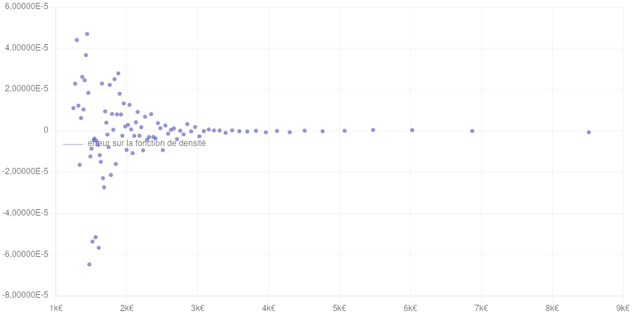
On constate que les erreurs entre notre modèle et le jeu de validation sont minimales lorsque  et
et  .
.
Lorsque l’erreur maximale en valeur absolue peut être divisée jusqu’à 4 par rapport à  , tandis que l’erreur en valeur absolue moyenne peut quant à elle augmenter jusqu’à
  . Afin de minimiser l’erreur maximale, nous avons choisi .
Test avec les données de 2020
Points larges : données d’entraînement du modèle. Points petits : données de validation. Courbe : modèle de la fonction de répartition.
Points petits : taux d’accroissements calculés à partir des données de validation. Courbe : modèle de la fonction de densité obtenu par dérivation du modèle de la fonction de répartition.
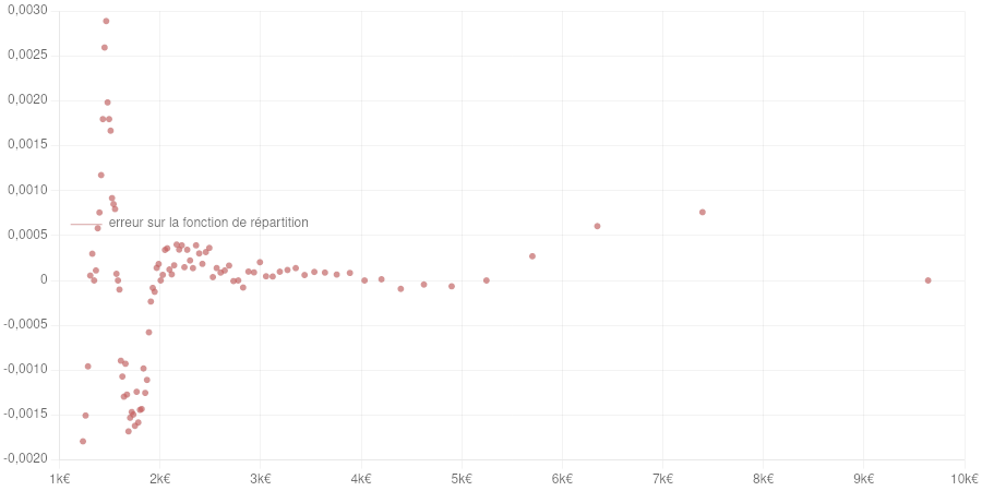
 ) et les données de validation fournies par l’INSEE.